
Machine learning is not reserved for men in lab coats. Great educational institutions do not harbor secret knowledge or skills. Machine learning can be done by anyone; you just need to know which knob to turn, and when.
If you’re a beginner, machine learning can feel overwhelming—how to choose which algorithms to use, from seemingly infinite options, and how to know just which one will provide the right predictions (data outputs). Of course, there are plenty of how-to’s and tutorials out there. Diving into these gives you glimpses of the whole.
In this article, I offer an overview of how all the parts fit together.
Like I can say a car is assembled from a set of tires, chassis, and an engine, and you know it’s not actually that simple, but a decent start overall, here I give something similar to Machine Learning models and their algorithms. This overview of ML algorithms offers a fine balance of:
- Ease
- Lower computational power
- Immediate, accurate results
We’ll cover: how ML works, tools you’ll use, ML types, layers of ML, and finally, the algorithms. At the end, I’ll also recommend additional resources for your ML journey. Let’s get started!
How ML works
Machine learning is a branch of statistics, specifically geared towards modelling. Machine learning models are capable of “learning” by:
- Making a prediction
- Testing the prediction
- Measuring the error
- Modifying the weights of the model to try and decrease the error (all the nodes in the hidden layer)
- Making a new prediction
Machine Learning iterates on this cycle over and over and over. This iterative cycle is the resource-rich component of ML. The data gets passed around on the computer, the model itself has a size, and the back propagation step that readjusts the model’s weights all take computer resources.
Then, when those steps get repeated thousands (or billions) of times over, that can cost a lot of computational resources.
Tools to get started
The Keras library is a Python package designed to handle a lot of the underlying details for ML engineers. It provides out-of-the-box models to handle some of the basic modelling needs. It is built on top of TensorFlow. TensorFlow, PyTorch, and SciKit Learn are a few of the largest machine learning libraries, with a shift in preference moving towards PyTorch.
If you get started with Machine Learning, likely you’ll be using one of these frameworks and writing your code in Python.
Types of machine learning
At its most basic, machine learning is a way for computers to run various algorithms without direct human oversight in order to learn from data. Machine learning can include running any variety of tasks in order for the machine to determine a high-probability outcome for various information, such as:
- The functions between input and output
- The hidden structures in unlabeled data
In instance-based learning, the machine can produce class labels by comparing previous instances. These ways of learning are summed up in the three types of machine learning algorithms:
Supervised learning
Supervised learning methods rely on labeled training data sets to learn a function between input variables (X) and output variables (Y). The most common types include:
- Classification methods, which predict the output of a given data sample when the output variable fits into one category, for instance dead or alive, sick or healthy.
- Regression methods, which predict output variables that are real values, such as the age of a person or the amount of snowfall.
- Ensemble methods, which combine predictions from weaker algorithmic output to predict new output.
Unsupervised learning
These methods use only input variables (X), not output variables, and rely on unlabeled training data sets to map the underlying structure of the data. Common examples include:
- Association methods, which uncover probability of items in a collection, as in market-basket analysis.
- Clustering methods, which group samples of objects based on similarity.
Reinforcement learning
Reinforcement learning methods allow the user or other designated agent to decide the best next action, based on the current state and learned behaviors that maximize the rewards. This approach is common in robotics.
Machine learning layer by layer
The technical elements of Machine Learning are:
- Data inputs
- Model layers
- An activation function
- An output layer
- Back propagation method

Given these five things, you can build a machine learning model. These five things each have a lot that can be known about them, and, like a well-constructed watch, all five parts need to coordinate and cooperate with one another in order for the whole model to work.
Let’s look at each piece in detail.
Preprocess your data
After determining the type of learning (above) that needs to happen on your data, building the Machine Learning Model algorithms begins with the pre-processing step. You’ll need to configure your data to work with the model.
All data can be placed into one of two categories, and how it moves down the pipe depends which category it gets placed into:
- Categorical: Nominal or ordinal
- Numerical: Discrete or continuous
If there are lots of tasks in this preprocessing step, this step is often known as the data pipeline—the data changes as it goes down the pipe. If you are actively changing data to fit into a model, that is called feature engineering. The data can consist of different types like image data and text data.
The input & model layers
We can demystify the otherwise symbolic first layer of the neural network. The input layer is literally the data that’s input into the model.
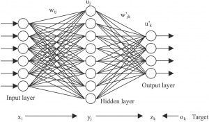
The number of nodes in the input layer on the neural network diagram corresponds exactly to the number of features of data. If you used age data, education data, and income data to predict how many airplane flights one will take in a lifetime, then that is three data features, and would be represented as three nodes in the neural network graph.
Now, images or language can’t be processed directly by the model, so they get transformed in the data pipeline by a number of encoding methods to convert either colors or language into a series of numbers for the model to be able to work with.
Popular encoding methods are:
- One-hot encoding
- Label encoding
- TF-IDF vectors
The activation layer
Every machine learning model is composed of layers. The activation layer is the step that converts the hidden layer’s values into the output. The activation layer is responsible for returning an output such as Cat or Dog, 0 or 1, or, instead of a hard label, it can return a percentage like .45.
There are many, many kinds of activation layers and their use will vary based on what kind of problem is being solved.
Curves of some activation functions look like this:
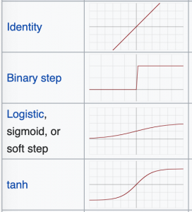
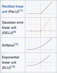
Based on the curves, you can see how the activation function creates a set of possibilities for the outputs. So, you can pick the activation based on which possibilities you wish to see in the output. I will explain.
- If the output needs to be an either/or output like a classifier, then a binary step function or ReLU may work because it returns one number or another.
- If you need numbers between two limits like 0 or 1, or -1 and 1 then tanh or the sigmoid functions are your go-tos because they allow a range of possibilities between those limits.
Sometimes, modelers will require the percentage of their function to be over X% in order to label their output as a single entity.
The output layer & back propagation
Finally, let’s demystify the last layer of the neural network. The “output layer” is literally the data returned from the activation function.
- If the activation function returns an either/or response, then it will be graphed as two nodes.
- If the model is a multi-label classifier and can return eight different kinds of labels, then the final output layer on the graph will be drawn with eight nodes.
The learning element of machine learning, which separates machine learning from other non-algorithm-based models, is the back propagation step. This one step single-handedly allows a model to learn by
- Calculating the error of the model’s predictions.
- Fine-tuning the weights of the model back in the hidden layer to make a more accurate prediction.
The model’s ability to learn relies on its ability to predict a known value, measure its error, then reconfigure its weights so that, on the next prediction, the model can make a better prediction. Back propagation is entirely responsible for the “learning” element of machine learning.

Back propagation deals with the idea of gradient descent. Imagine an empty swimming pool or the bowl at a skatepark. You begin on its edges, and you have to take one step at a time to reach its lowest point; that would be gradient descent. A model’s prediction will have an error, and a surface can be made from that error function. The lowest point on the surface will be the point with the lowest error.
If you are on the edge of the swimming pool, far from the lowest point, you exist in a space where the model’s predictions are very wrong. If you are inches from the drain, you are very close to making accurate predictions.
The major adjustable component for any ML newbie is tweaking the learning rate (alpha). This learning rate tells the algorithm how big each step should be to reach the lowest point.
There is a risk with being too small or too large. Small steps mean it can take a very long time to inch towards the lowest point, and large steps mean you can actually overshoot it and go out the other side of the pool.
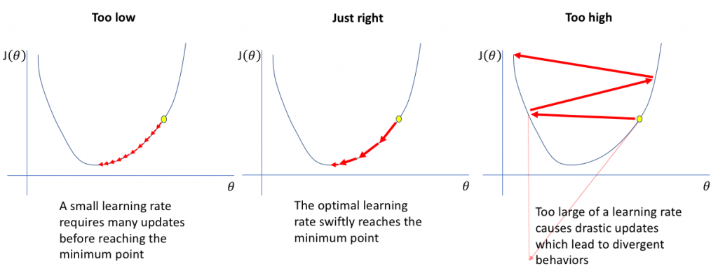
(Source)
These are the basics to the back propagation step. The surface, the way the errors are visualized, can grow more technical.
Popular ML algorithms for beginners
The construction of the model’s layers define what kind of algorithm is going to be used. There are four main tasks machine learning solves:
- Regression predicts an outcome.
- Classification labels a piece of data.
- Generation uses data to generate like-data.
- Sequencing predicts the next element in a sequence.
Now, let’s look at some specific algorithms that fall into these categories.
Linear regression
Despite its name, linear regression is a classification method, not a regression method. This predictive modeling approach is very well understood—statistics has been using this tool for decades before the invention of the modern computer.
The goal of linear regression is to make the most accurate predictions possible by finding the values for two coefficients that weight each input variable. These techniques can include:
- Linear algebra
- Gradient descent optimization
- And others
Employing linear regression is easy and generally provides very accurate results. More experienced users know to remove variables from your training data set that are closely correlated and to remove as much noise (unrelated output variables) as possible.
To employ a simple linear regression model in Keras, the python code looks like this. And as ML expert Aurélien Géron points out, the main difference between this linear regression and a classification model is on the output layer.
The line keras.layers.Dense(1) has only one output neuron, and we see, here, the activation function that’s used is the “relu”.
model = keras.models.Sequential([
keras.layers.Dense(30, activation="relu", input_shape=X_train.shape[1:]),
keras.layers.Dense(1)
])
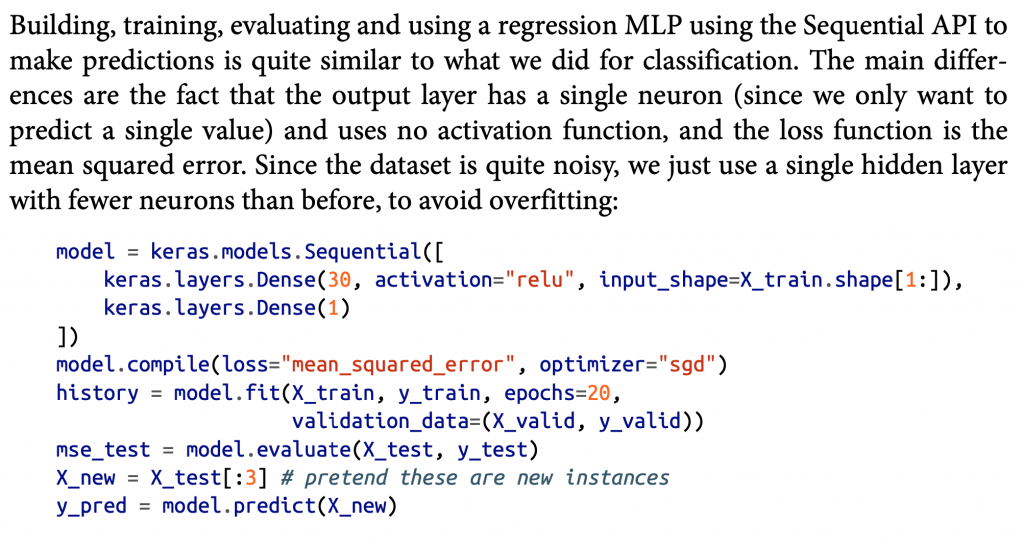
(Géron’s Hands On Machine Learning with SciKit 2e, pg. 303)
Logical regression
Similar to linear regression, logical regression is another statistical method for classification that finds the values for two coefficients that weight each input variable.
The difference is that this solves problems of binary classification, relying on a logical, non-linear function instead. Therefore, logical regression determines whether a data instance belongs to one class or another and can also provide the reason behind the prediction, something linear regression cannot do.
When using this algorithm, limiting correlating data and removing noise is important.
Classification
Classification and regression trees are easy to learn and use, and they’re accurate for a whole range of problems. These are especially speedy to implement, as the data requires no special preparation.
More data is better for machine learning models, so, where possible—image data, for example—instead of needing to one-hot encode a data input, modelers will try to create similar data points from the given ones.
For our example of images, images in the dataset can be flipped, blurred, cut, mirrored, stretched many different ways to get more data, and more specifically, more labelled data. If the image was a dog before the image was blurred a bit, then it is still a dog after.
The most common Neural Network architecture for classification is the Convolutional Neural Network (CNN).
Classification in a Neural Network looks like this:
model = keras.models.Sequential()
model.add(keras.layers.Flatten(input_shape=[28, 28]))
model.add(keras.layers.Dense(300, activation="relu"))
model.add(keras.layers.Dense(100, activation="relu"))
model.add(keras.layers.Dense(10, activation="softmax"))
(Ibid, pg. 295)
Compared to the linear regression algorithm, this has two hidden layers inside it using the ReLu activation function and a final softmax activation on the output layer. The two middle layers have 300 and 100 nodes respectively.
The input layer is an image that is 28 pixels wide by 28 pixels tall. The input layer is told to flatten the 28×28 image and each pixel gets a node on the input layer. 28 * 28 = 784, so there will be 784 nodes as the input layer.
This classification model was built for the MNIST data which classifies a handwritten digit as 0-9. Since there are 10 possible outcomes, the output layer has 10 available nodes.
K-nearest neighbor (KNN)
With the K-nearest neighbor method, the user specifies the value of K. Unlike previous algorithms, this one trains on the entire dataset.
The goal of KNN is to predict an outcome for a new data instance. The algorithm trains the machine to check the entire dataset to find the k-nearest instances to this new data instance or to find the k-number of instances that are most similar to the new instance. The prediction, or output, is one of two things:
- The mode or most frequent class, in a classification problem
- The mean of the outcomes, in a regression problem
This algorithm usually employs methods to determine proximity such as Euclidean distance and Hamming distance. Euclidean distances are the kinds of distances that everybody learns in early education. It maintains that the shortest distance between two points is a straight line. (In other geometries, this statement becomes false.)
KNN works like this. When a bunch of data is thrown on the table, the KNN algorithm begins to sort each into separate categories.

(Source)
A person employs the KNN algorithm when solving a 500-piece puzzle. Typically, you’ll dump the pieces on a table and place each piece (a piece of data) into a category, an easily identifiable color or object on the final image. By sifting and ordering, over and over, pieces that share the same color get closer and also get placed further from unlike colors.
The advantages of KNN are:
- Simplicity
- Ease of use
Though it can require a lot of memory to store large datasets, KNN only calculates (learns) at the moment a prediction is needed.
When using a high number of input variables, the machine-learned understanding of “closeness” can be compromised. This situation, known as the curse of dimensionality, can be avoided by limiting your input variables to only those that are most relevant to predicting the output.
Naïve Bayes
Like other beginner algorithms, the Naïve Bayes algorithm is a classifier that uses training data in a simple manner with powerful outputs. Naïve Bayes employs the Bayes theorem of probability to classify content. The Bayes Theorem calculates probability of an event occurring or a hypothesis being true based on prior knowledge, making the model able to handle two types of probabilities:
- Determining class
- Determining a conditional probability of each class, provided X value
Importantly, the “naïve” part of the title is based on the algorithm’s assumption that the variables are independent of each other, which is often unrealistic in real-world examples.
The content best suited for this Naïve Bayes is often language-based, such as:
- Web pages
- Articles
- Smaller bodies of text, like tweets or metadata from blogs
This algorithm is a go-to option when trying to rank content or classify data based on categories (content themes). This algorithm has also been used effectively in:
- Predicting disease development and location
- Analyzing human sentiment
Learning materials
That concludes this overview of machine learning algorithms. Here are some learning materials I’ve used and recommend to you:
Online courses
- Andrew Ng’s ML Coursera (The quintessential ML course)
- A-Z Deep Learning from Udemy
- MITx
Book
- Aurélien Géron’s Hands-On Machine Learning with Scikit-Learn, Keras, and TensorFlow: Concepts, Tools, and Techniques to Build Intelligent Systems 2nd Edition
BMC resources
- BMC Machine Learning & Big Data Guide
- BMC Guides for TensorFlow, Keras, scikit-learn, Data Visualization, and more
- Machine Learning Architectures Explained
- Interpretability vs Explainability: The Black Box of Machine Learning
- Containerized Machine Learning: An Intro to ML in Containers
These postings are my own and do not necessarily represent BMC's position, strategies, or opinion.
See an error or have a suggestion? Please let us know by emailing blogs@bmc.com.