
Here we explore another machine learning framework, scikit-learn, as well as show how to use matplotlib, to draw graphs. Check out the official site for scikit-learn.
The scikit-learn python ML API predates Apache Spark and TensorFlow, which is to say it has been around longer than big data. It has long been used by those who see themselves as pure data scientists, as opposed to data engineers. Still you can connect scikit-learn to Spark so that the transformations and calculations you can run across a cluster of machines. Without that you can only work with datasets that fit into the memory, cpu speed, and disk space of a single machine.
Scikit-learn is very strong on statistical functions and packed full of almost every algorithm you can think of, including those that only academics and mathematicians would understand, plus neural networks, which is applied ML. But you need not be a mathematician to get started with the product. Here we show how to code the simplest possible example.
(This article is part of our scikit-learn Guide. Use the right-hand menu to navigate.)
Environment
You should use conda to setup Python and install packages. This will make it easy to integrate sckit-learn with Zeppelin Notebooks. It is difficult to add python packages to Zeppelin otherwise.
You could run this example from the Python command line, but Zeppelin is graphical, so you can draw nice graphs with matplotlib.
When you install Zeppelin, install the package with ALL interpreters so that Python, Spark, matplotlib. etc. are there. Follow this example if you are new to Zeppelin to understand that.
Install Anaconda and then enter this command to install scikit-learn:
conda install scikit-learn
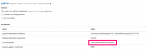
Then in Zeppelin point your Python interpreter to the Anaconda Python like this:
Example
We will do the simplest possible example, which is linear regression with 1 independent variable and 1 dependant variable. And we will set up our data so that the data is perfectly correlated, meaning the variance is 1. In other words, with LR the goal is to solve this equation for a straight line by finding the coefficient m and y intercept b.
y = mx + b
But our goal here is just to show how to use scikit-learn. So we will mock our data using y = 2x + 0 = 2x. (If you want a more realistic example you could use the standard normal distribution and draw a random noise factor from that and add that to y.)
The code from this example is stored here as a Zeppelin notebook. Below we show the code in sections. You can paste the sections into Zeppelin paragraphs in a Zeppelin notebook. Be sure to select the python interpreter when you create the notebook.
import matplotlib.pyplot as plt
from sklearn import linear_model
import numpy as np
from sklearn.metrics import mean_squared_error, r2_score
First we instantiate the LinearRegression model.
reg = linear_model.LinearRegression()
Next we make an array. On the left are the independent variables 1,2,3. On the right are the dependant ones 2,4,6. As you can see each dependent variable y is equal to each dependant variable x times 2, i.e., y=2x.
Scikit-learn expects you to use a numpy array.
ar = np.array([[[1],[2],[3]], [[2],[4],[6]]])
ar
Results. Printing out each result helps to visualize and understand it.
array([[[1],
[2],
[3]],
[[2],
[4],
[6]]])
Here we slice the array taking just the y variables. (Slicing and reshaping arrays is a complicated topic. You can read about that here.) This array shape, ar.shape, is given in this tuple (2,3,1). This is an array 1 of 2 arrays. So we alternatives take the first 1 x 3 array at the second position for y:
y = ar[1,:]
y
Results:
array([[2],
[4],
[6]])
Then take the first one for x.
x = ar[0,:]
x
Results:
array([[1],
[2],
[3]])
Now we have the independent variables stored in a simple vector x and the dependant variables in y. In terms of machine learning we say we have 1 feature and 1 label.
Now we run fit() which uses the least squares method to find the line y=mx, by finding the slope m, which is the same as saying the coefficient m for the line y = mx.
reg.fit(x,y)
Now we can print the coefficient from the linear regression API.
print('Coefficients: \n', reg.coef_)
Result is 2, which we would expect since we know the line is y = 2x.
Coefficients:
[[2.]]
Now let’s make test data the same way, 4,5,6 and then 2 times that for y:
xTest = np.array([[4],[5],[6]])
xTest
Results:
array([[4],
[5],
[6]])
Now feed the x test values xTest into predict method. It will return an array of y prediction.
ytest =  np.array([[8],[10],[12]])
preds = reg.predict(xTest)
preds
Results:
array([[ 8.],
[10.],
[12.]])
Now look at the error, which is the difference between the observed values (ytest) and predicted (preds). Of course, it is zero.
print("Mean squared error: %.2f" % mean_squared_error(ytest,preds))
Results:
Mean squared error: 0.00
And the variance is 1, since the data is perfectly correlated.
print("Variance score: %.2f" % r2_score(ytest,preds))
Results
Variance score: 1.00
Now we can plot is using matplotlib:
plt.scatter(xTest,preds, color='black')
plt.plot(xTest,preds,color='blue', linewidth=3)
plt.show()
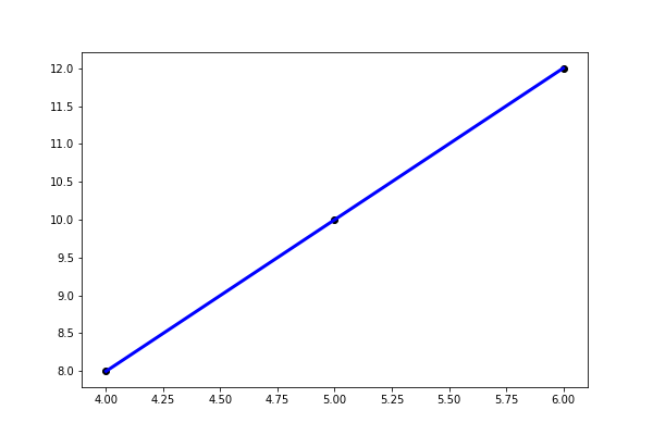
That is the simplest possible example of how to use scikit-learn ML library to do linear regression.
These postings are my own and do not necessarily represent BMC's position, strategies, or opinion.
See an error or have a suggestion? Please let us know by emailing blogs@bmc.com.