
NumPy supports many statistical distributions. This means it can generate samples from a wide variety of use cases. For example, NumPy can help to statistically predict:
- The chances of rolling a 7 (i.e, winning) in a game of dice
- How likely someone is to get run over by a car
- How likely it is that your car will breakdown
- How many people will be in line at the checkout counter
We explain by way of examples.
(This tutorial is part of our Pandas Guide. Use the right-hand menu to navigate.)
Randomness & the real work
The NumPy functions don’t calculate probability. Instead they draw samples from the probability distribution of the statistic—resulting in a curve. The curve can be steep and narrow or wide or reach a small value quickly over time.
Its pattern varies by the type of statistic:
- Normal
- Weibull
- Poisson
- Binomial
- Uniform
- Etc.
Most phenomena in the real world are truly random. For example, if we toss out nearsightedness, clumsiness, and absentmindness, then the chance that someone would get hit by a car is equal for all peoples.
The normal distribution reflects this.
When you use the random() function in programming languages, you are saying to pick from the normal distribution. Samples will tend to hover about some middle point, known as the mean. And the volatility of observations is called the variance. As the name suggests, if it varies a lot then the variance is large.
Let’s look at these distributions.
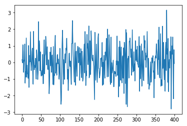
Normal
The arguments for the normal distribution are:
- loc is the mean
- scale is the square root of the variance, i.e. the standard deviation
- size is the sample size or the number of trials. 400 means to generate 400 random numbers. We write (400,) but could have written 400. This shows that the values can be more than one dimension. We are just picking numbers here and not any kind of cube or other dimension.
import numpy as np
import matplotlib.pyplot as plt
arr = np.random.normal(loc=0,scale=1,size=(400,))
plt.plot(arr)
Notice in this that the numbers hover about the mean, 0:
Weibull
Weibull is most often used in preventive maintenance applications. It’s basically the failure rate over time. In terms of machines like truck components this is called Time to Failure. Manufacturers publish for planning purposes.
A Weibull distribution has a shape and scale parameter. Continuing with the truck example:
- Shape is how quickly over time the component is likely to fail, or the steepness of the curve.
- NumPy does not require the scale distribution. Instead, you simply multiply the Weibull value by scale to determine the scale distribution.
import numpy as np
import matplotlib.pyplot as plt
shape=5
arr = np.random.weibull(shape,400)
plt.hist(arr)
This histogram shows the count of unique observations, or frequency distribution:

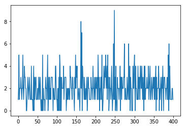
Poisson
Poisson is the probability of a given number of people in the lines over a period of time.
For example, the length of a queue in a supermarket is governed by the Poisson distribution. If you know that, then you can continue shopping until the line gets shorter and not wait around. That’s because the line length varies, and varies a lot, over time. It’s not the same length all day. So, go shopping or wander the store instead of waiting in the queue.
import matplotlib.pyplot as plt
arr = np.random.poisson(2,400)
plt.plot(arr)
Here we see the line length varies between 8 and 0, The number function does not return a probability. Remember that it returns an observation, meaning it picks a number subject to the Weibull statistical cure.
Binomial
Binomial is discrete outcomes, like rolling dice.
Let’s look at the game of craps. You roll two dice, and you win when you get a 7. You can get a 7 with these rolls:
- 1,6
- 2,5
- 3,4
- 4,3
- 5,2
- 6,1
So, there are six ways to win. There are 6*6*36 possibilities. So, the chance of winning is 6/16=⅙.
To simulate 400 rolls of the dice, use:
import numpy as np
import matplotlib.pyplot as plt
arr = np.random.binomial(36,1/6,400)
plt.hist(arr)
In the 400 trials, two 6s were rolled about three times.

Uniform
Uniform distribution varies at equal probability between a high and low range.
import numpy as np
import matplotlib.pyplot as plt
arr = np.random.uniform(-1,0,1000)
plt.hist(arr)